Page 18 - Code & Click - 7

4

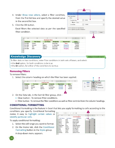
4. Under Show rows where, select a filter condition,
from the first list box and specify the desired value
in the second list box.

5. Click the OK button.
Excel filters the selected data as per the specified

filter condition.

5

Knowledge Discovery Subject Enrichment
To filter data on two conditions, enter filter conditions in both sets of boxes, and select:
• the And option, for both conditions to be true.
• the Or option, for either of the conditions to be true.

Removing Filters
To remove filters:
1. Select the column heading on which the filter has been applied.

1
2. On the Data tab, in the Sort & Filter group, click :
• Clear button : To remove filter conditions.
• Filter button : To remove the filter conditions as well as filter controls from the column headings.

CONDITIONAL FORMATTING
Conditional Formatting is the feature in Excel that lets you apply formatting to cells according to the
conditions you specify. Conditional formatting
makes it easy to highlight certain values or
identify particular cells.
To apply conditional formatting:

1. Select the cell range you want to format.
2. On the Home tab, click the Conditional
Formatting button in the Styles group.
A drop-down menu appears.

16