Page 79 - Physics - XI

Plotting of Data with Error Bars
5. Now, put the marking of points of the loads on the load axis and of extension on the extension axis of

the graph paper.
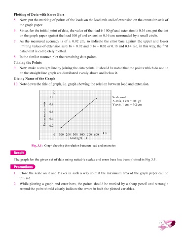
6. Since, for the initial point of data, the value of the load is 100 gf and extension is 0.16 cm, put the dot
on the graph paper against the load 100 gf and extension 0.16 cm surrounded by a small circle.
7. As the measured accuracy is of ± 0.02 cm, so indicate the error bars against the upper and lower

limiting values of extension as 0.16 + 0.02 and 0.16 – 0.02 or 0.18 and 0.14. So, in this way, the fi rst
data point is completely plotted.
8. In the similar manner, plot the remaining data points.

Joining the Points
9. Now, make a straight line by joining the data points. It should be noted that the points which do not lie
on the straight line graph are distributed evenly above and below it.
Giving Name of the Graph

10. Note down the title of graph, i.e. graph showing the relation between load and extension.

Y
1.0 Scale used:
X-axis, 1 cm = 100 gf
0.8 Y-axis, 1 cm = 0.2 cm
Extension (cm) 0.6

0.4

0.2

0 100 200 300 400 500 600 X
Load (gf)

Fig. 3.1: Graph showing the relation between load and extension

Result

The graph for the given set of data using suitable scales and error bars has been plotted in Fig 3.1.

Precautions

1. Close the scale on X and Y axes in such a way so that the maximum area of the graph paper can be
utilised.
2. While plotting a graph and error bars, the points should be marked by a sharp pencil and rectangle

around the point should clearly indicate the errors in both the plotted variables.

77