Page 261 - Ai Book - 10

In the figure, you can see the four images in which the visual appearance of each image is different. This is
tpossible only due to the changing in pixel values. The process of convolution and the convolution operator (*)
are commonly used to create these types of effects or changing the pixel values evenly throughout the image.
Let us understand the theory of convolution through the following definitions.
In general, the Convolution technique is used for general signal processing. Convolution, a technical term
refers to a process of multiplying together two arrays of numbers, generally of different sizes, but of the
same dimensionality, to produce a third array of numbers of the same dimensionality. In image processing, a
convolution requires three components:An input image, a kernel matrix that we are going to apply to the input
image, an output image to store the output of the input image convolved with the kernel.
KERNEL MATRIX

A small matrix used to apply effects such as the ones you might find in Photoshop or Gimp, i.e. blurring,
sharpening, outlining or embossing is called image kernel. A kernel matrix can also be used in machine learning
for ‘feature extraction’, a technique for determining the most important portions of an image.
As you have read earlier, a kernel matrix is commonly used in the process of convolution to extract certain
features from an input image. We will get the enhanced output image through the kernel matrix which is slid
across the image and multiplied with the input image. You should remember that if you want to apply different
kind of effects on an image, then each kernel has a different value.
2-D Convolution

In 2-D convolution, we convolve two different matrices. 2-D convolution is widely used in image processing for
filtering, edge detection, and smoothing applications. One matrix is the image matrix. The other is called the
Kernel (which performs a specific function). The convolution will produce the desired output, 2-D convolution
is also performed in the same manner as 1-D convolution. We keep the input image matrix as it is, invert the
Kernel matrix and then slide the Kernel matrix over the input image matrix. We’ll match the centre of the Kernel
matrix with each value of the input matrix, one by one, and calculate the output for the corresponding location
by calculating the sum of products of intersections.
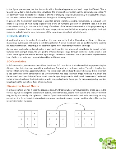
Flipping the Kernel Matrix

In 1-D convolution, we had flipped the sequence once. In 2-D convolution, we’ll reverse it two times. Once in the
vertical flip, we exchange the top row with bottom, second from top, second from buttom and so on. In the next
step, we flip horizontally. The rightmost column is flipped with the leftmost and so on for the remaining. For easy
operations, the Kernel matrix is always kept as a square matrix with rows = columns = odd numbers. The number
is 3 or 5 in most of the cases.

1 2 3 3 2 1 9 8 7

4 5 6 6 5 4 6 5 4

7 8 9 9 8 7 3 2 1

135
135